
Neon: Building a Trustworthy Solver-Plus-ML Research Platform for Nanophotonics
I started Neon because I wanted a research codebase I could understand end to end — and because I was skeptical of most surrogate modeling papers I was reading.
The literature on machine learning for photonics has grown rapidly since Peurifoy et al. demonstrated in 2018 that neural networks could predict the scattering properties of multilayer nanoparticles far faster than direct simulation [1]. Since then, dozens of papers have trained networks on electromagnetic simulation data, reported strong accuracy numbers on held-out test sets, and moved on. What most of them do not report carefully: what happens outside the training distribution, whether the physics-informed losses actually earn their computational cost, whether uncertainty estimates are calibrated, and whether a better surrogate actually finds better designs.
Those are the questions Neon was built to answer, on a controlled benchmark, without overclaiming. This post is a completed-work summary. The codebase is stable, the experiments are done, and a paper is in preparation.
Background: The Surrogate Modeling Problem in Photonics
The core challenge is well understood. Rigorous electromagnetic simulation — whether finite-difference time-domain (FDTD) as in Oskooi et al.’s Meep [2], finite-difference frequency-domain (FDFD), or high-order discontinuous Galerkin methods as in the DIOGENeS suite from Inria’s Atlantis team [3] — is computationally expensive. A single solve on a modest 2D grid can take seconds; a full inverse-design sweep over thousands of configurations can take hours or days. This makes brute-force parameter search impractical and motivates surrogate-based approaches.
The surrogate idea is straightforward: train a neural network on a dataset of simulation inputs and outputs, then use the network instead of the full solver during design search. The network is wrong sometimes, but it is thousands of times faster. If you then verify only the most promising candidates with the direct solver, the total simulation budget shrinks dramatically.
This idea has been explored across many photonic problem classes. Liu et al. [4] trained tandem networks for metasurface design. Wiecha et al. [5] gave a broad review of deep learning in nanophotonics covering both forward prediction and inverse design. So and Bravo-Abad [6] reviewed the landscape specifically from the lens of inverse design. The accuracy numbers reported across these works are often impressive. What is reported less often is why the model works where it does, what happens when it encounters structures outside the training set, and whether the reported accuracy translates into better design outcomes.
The physics-informed neural network (PINN) framework, introduced rigorously by Raissi, Perdikaris, and Karniadakis in 2019 [7], offered a natural way to incorporate governing equations directly into training. By adding a PDE residual term to the loss function, the network is penalized not just for fitting the data badly but for producing outputs that violate the physics. For electromagnetic problems, this has attracted significant interest — if physics constraints can substitute for data, maybe we need fewer expensive simulations to train a reliable surrogate.
That is the hypothesis Neon was built to test carefully. Not to implement a PINN and call it done, but to check whether the physics terms actually earn their place under controlled ablation.
What Neon Is
Neon is a C++ scalar frequency-domain Helmholtz solver with a Python/PyTorch ML layer built on top of it. It is not a general Maxwell solver. It is a research platform for careful, small-scope benchmarking.
The governing equation is the scalar out-of-plane Helmholtz model:
\[\nabla^2 E_z(x, y) + k_0^2 \varepsilon_r(x, y) E_z(x, y) = s(x, y), \qquad k_0 = \frac{2\pi}{\lambda}\]This is a 2D, monochromatic, scalar formulation — the same class of reduced model used in many photonics surrogate benchmarks because it retains physically meaningful structure (resonance behavior, transmission and reflection, field concentration) while remaining computationally tractable enough to generate large datasets and run controlled ablations. The solver assembles a sparse finite-difference system on a structured Cartesian grid and solves it using Eigen’s SparseLU, with an optional iterative BiCGSTAB path. The current benchmark family is a parameterized rectangular dielectric slab in vacuum at normal incidence.
On top of this solver, Neon builds a complete ML experimentation layer: solver-driven dataset generation, baseline surrogate training, hybrid physics-informed training, deep ensemble uncertainty, active learning, and inverse design screening — all driven by the same direct solver outputs, with direct solver reevaluation mandatory at every design stage.
The codebase is now live at https://github.com/Herr-Professor/Neon and the trained model is available at https://huggingface.co/Herrprofessor/Neon.
The Solver: Validation Before ML
A core design principle of Neon is that the direct solver must be validated before any ML layer is trusted. This sounds obvious, but it is easy to skip in practice: if the solver produces outputs that are wrong in a systematic way, every surrogate trained on those outputs learns to predict the wrong thing confidently.
Absorber Treatment
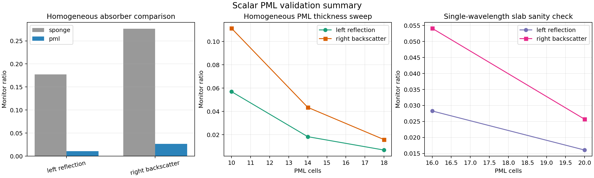
The first major solver upgrade was boundary treatment. Neon’s original sponge absorber — a gradually increasing imaginary permittivity layer that damps outgoing waves — is simple to implement but introduces significant spurious reflections. The standard improvement is the Perfectly Matched Layer (PML), originally introduced for time-domain Maxwell equations by Bérenger [8] and extended to stretched-coordinate formulations by Chew and Weedon [9].
Neon implements a scalar stretched-coordinate PML for the current Helmholtz formulation:
\[\partial_x \left( \frac{s_y}{s_x} \partial_x E \right) + \partial_y \left( \frac{s_x}{s_y} \partial_y E \right) + k_0^2 \varepsilon_r s_x s_y E = s_x s_y f\]where $s_x$ and $s_y$ are the complex stretching functions. This is not a general Maxwell PML — it is specifically derived for the current scalar Helmholtz formulation, and the outer boundary is still Dirichlet-terminated. But it is materially better than the legacy sponge on the current benchmark. The left reflection ratio drops from 0.1772 to 0.0109 — a 16.3x reduction — and the right-side backscatter ratio drops from 0.2765 to 0.0266, a 10.4x reduction.
External Validation: The TMM Lesson
Once the absorber was in better shape, I wanted to compare Neon’s outputs against an external analytic reference. The Transfer Matrix Method (TMM) is the natural choice for a slab geometry: it gives exact transmission and reflection coefficients for planar multilayer structures at normal incidence, derivable directly from Maxwell’s boundary conditions [10].
The first comparison failed badly: mean absolute error of 0.228 in transmission. But the failure was instructive. The signed bias was consistently positive — meaning Neon was systematically overestimating transmission relative to TMM, not scattering randomly around the right answer. That pattern is characteristic of a normalization or output-quantity mismatch, not a solver error.
The root cause was that Neon’s transmission and reflection values were monitor-based proxies: local field amplitude samples decomposed heuristically into forward and backward components at a monitor line. These are useful diagnostics, but they are not rigorous flux-normalized power coefficients. After implementing a proper benchmark-facing scalar normalization for the current lossless normal-incidence slab family, the TMM comparison improves to a mean absolute error of 0.0489 and now passes.
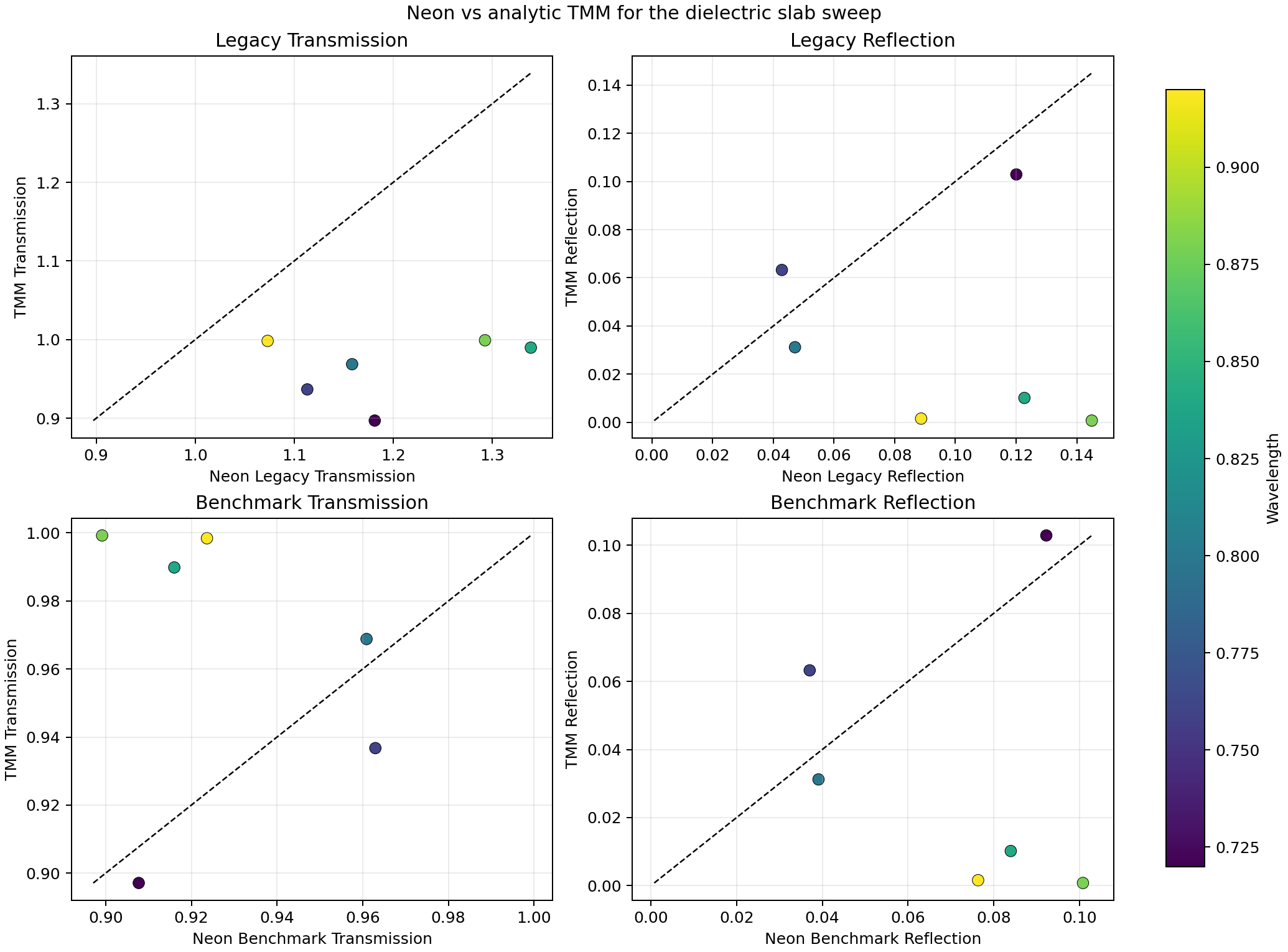
The lesson is general: output quantity definition matters as much as model architecture when training surrogates. A network trained on a systematically biased output quantity will learn the bias, not the physics.
A cross-check against Ceviche [11] — a differentiable FDFD solver developed by Tyler Hughes and colleagues at Stanford — is less clean. Even after correcting a methodology error (comparing $E_z$ to $E_z$ rather than $E_z$ to $H_z$), the field magnitude correlation is 0.8737. This discrepancy is not yet resolved. It could be grid resolution differences, PML padding mismatches, or source-placement conventions between the two codes. I keep this result in the repository as a documented open question, not a swept-under-the-rug failure.
The ML Layer: Three Models, One Question
The ML experimentation ladder in Neon has three levels, each adding something to the training formulation.
Model A is a small PyTorch MLP taking slab thickness, relative permittivity, and wavelength as inputs and returning transmission, reflection, and peak intensity. No physics in the loss. Trained from scratch on 72 simulation samples from 12 slab designs. This is the baseline against which everything else is measured.
Model B adds a centerline field prediction and a physics-informed loss term: a reduced 1D Helmholtz residual computed along the centerline field, away from crop edges and slab interface points. This connects to the broader PINN framework of Raissi et al. [7] but is deliberately more modest: it applies only along a 1D cropped centerline, not the full 2D domain, and it uses precomputed solver fields rather than requiring the network to satisfy the PDE from scratch.
Model C extends Model B with two additional physics-derived penalties:
- A boundary-aware loss that penalizes backward-wave energy in a transmitted-side background window near the PML entrance region, derived from the same forward/backward decomposition used by the solver’s postprocessor.
- A source-aware loss that penalizes mismatch to the expected forward plane-wave structure in the source-side background region between the line source and the slab.
Both terms are genuinely physics-derived for this specific setup. Neither is a general Maxwell constraint. But they are real, not decorative.
The trained Neon model released on HuggingFace is the Model C checkpoint. It takes thickness, epsilon, and wavelength as inputs and returns transmission, reflection, and intensity:
from neon import Neon
model = Neon.from_pretrained()
result = model.predict(thickness=0.30, epsilon_real=2.25, wavelength=0.80)
# {"transmission": 0.87, "reflection": 0.09, "intensity": 1.31}
What the Results Actually Say
This is where the project becomes a benchmark platform rather than just a feature stack. The honest answer to “does adding physics to the loss function help?” is: sometimes, and not in the ways you might expect.
The A/B/C Comparison
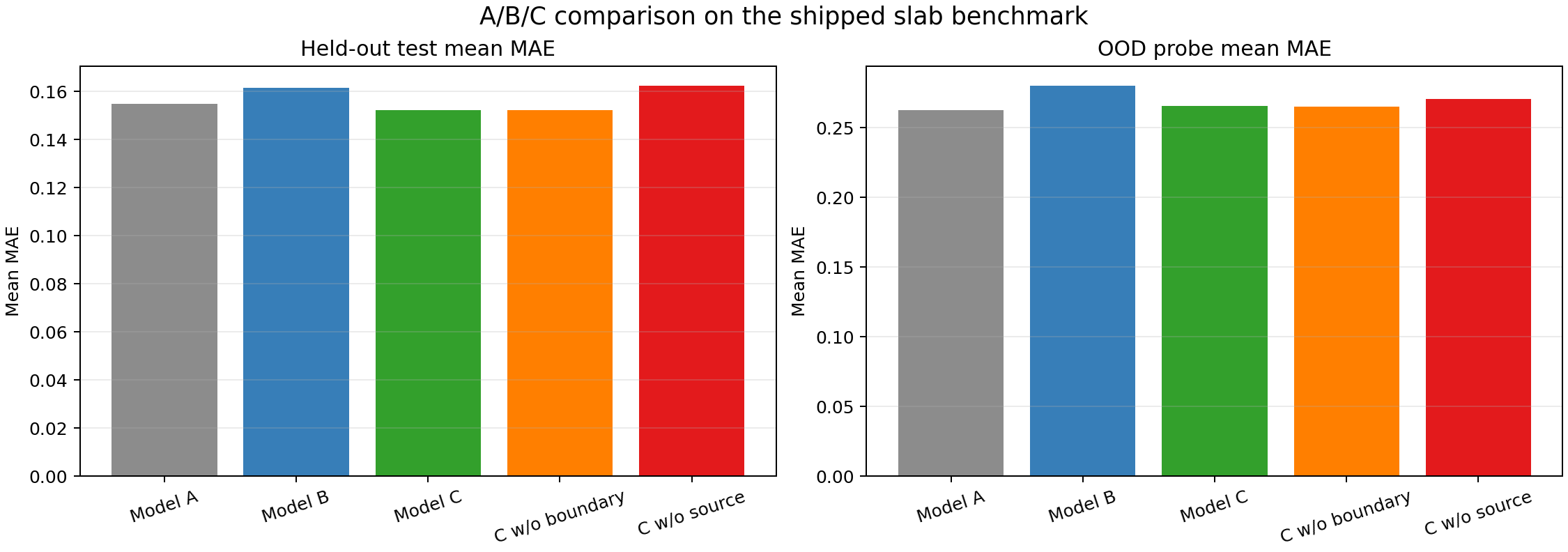
On the full 72-sample training set, the test mean MAEs are:
| Model | Test MAE | OOD MAE |
|---|---|---|
| A (baseline) | 0.1548 | 0.2627 |
| B (+ residual) | 0.1616 | 0.2802 |
| C (+ residual + boundary + source) | 0.1522 | 0.2653 |
Model C improves on both Model B and slightly on Model A on in-domain test error. It also improves on Model B on OOD. But it still does not beat the simple baseline on OOD — a finding that mirrors cautionary results in the broader physics-informed ML literature, where Krishnapriyan et al. [12] showed that naive PINN formulations can fail on relatively simple problems, and where Wang et al. [13] demonstrated that gradient pathologies in multi-term losses can prevent physics terms from contributing meaningfully.
The Ablation: What Is Actually Doing the Work
The component ablation is more informative than the headline comparison. Removing the source-aware term from Model C degrades test MAE from 0.1522 to 0.1625 and OOD MAE from 0.2653 to 0.2704. Removing the boundary-aware term changes almost nothing: 0.1522 to 0.1521 on test, 0.2653 to 0.2651 on OOD.
The source-aware term is doing real work. The boundary-aware term is nearly inert at full data.
This is a specific, interpretable finding. The source geometry — knowing where energy enters the domain, and what structure it should have there — is informative supervision that the data alone does not fully provide. The absorber-adjacent region, by contrast, does not carry enough additional signal beyond what the scalar targets already encode, at least in this reduced formulation.
This pattern connects to broader observations in the ML-for-PDE literature. Lagaris et al.’s original neural network approach to boundary value problems [14] showed that boundary conditions are often the hardest part to enforce. In Neon’s case, the source boundary is harder to ignore (it drives the whole field) and so a source-consistency penalty has more leverage than an absorber-exit penalty.
The Reduced-Data Study
The reduced-data ablation sweeps training set sizes from 2 to 12 slab designs across three random seeds:
| Train Designs | Model A MAE | Model B MAE | Model C MAE |
|---|---|---|---|
| 2 | 0.1723 | 0.1712 | 0.1734 |
| 4 | 0.1490 | 0.1392 | 0.1394 |
| 6 | 0.1673 | 0.1591 | 0.1579 |
| 8 | 0.1657 | 0.1651 | 0.1628 |
| 10 | 0.1640 | 0.1645 | 0.1623 |
| 12 | 0.1548 | 0.1616 | 0.1522 |
Model C beats Model B in 4/6 settings and beats Model A in 5/6 settings on in-domain test error. But at 2 training designs, Model C is worse than both. This is consistent with the known behavior of physics-informed losses identified by Rathore et al. [15]: physics constraints require enough data to orient themselves. In the extreme low-data limit, the regularization term competes with rather than complements the data term, because the network has not seen enough examples to place the physics constraint meaningfully in parameter space.
Model C beats Model A on OOD in exactly 0/6 settings. This is the most important result in the table. The physics terms help in-domain. They do not solve the extrapolation problem.
Uncertainty and Active Learning
The more recent additions to Neon address a different question: not whether to add physics to the loss, but whether the surrogate can tell you when not to trust it.
Deep Ensembles
The uncertainty approach follows Lakshminarayanan, Pritzel, and Blundell’s deep ensemble method [16]: train five independent MLPs with different random seeds, and use their disagreement as a proxy for predictive uncertainty. This is computationally cheap, does not require architectural changes, and has been shown to produce better-calibrated uncertainty than many more complex Bayesian approaches on tabular regression problems.
The current 5-member ensemble results are:
| Model | Test MAE | OOD MAE | Test σ | OOD σ |
|---|---|---|---|---|
| A ensemble | 0.1123 | 0.1172 | 0.0086 | 0.0212 |
| C ensemble | 0.1155 | 0.1293 | 0.0129 | 0.0258 |
Predictive spread does rise on OOD inputs for both models — the right qualitative behavior. But the uncertainty-error correlation is weak and inconsistent: -0.0087 on test for Model A, 0.2458 on OOD for Model C. This means the ensembles are useful as heuristics but cannot be described as calibrated in the sense of Kuleshov, Fenner, and Ermon [17], where calibration requires that stated confidence intervals actually contain the true value at the stated frequency.
Active Learning
The active learning workflow follows the standard uncertainty-guided acquisition approach: at each round, evaluate ensemble uncertainty across the full parameter grid, run the direct solver on the highest-uncertainty configuration, add that sample to the training set, and retrain. This connects to the broader active learning literature summarized by Settles [18] and to recent work on active learning for scientific simulation by Lookman et al. [19].
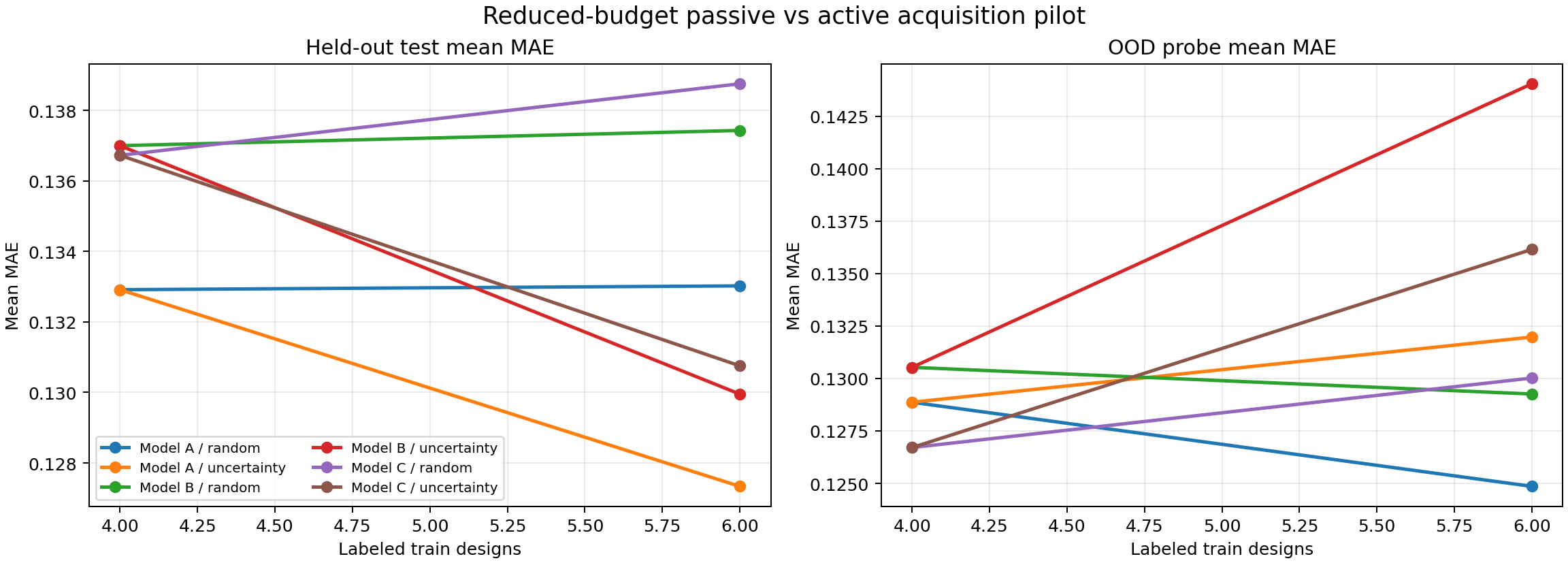
The shipped comparison uses one acquisition seed, 4 initial training designs, and one round adding 2 more designs — a deliberately reduced budget, reported honestly as a pilot rather than a full study.
Results at this budget:
| Model | Test MAE (active) | Test MAE (passive) | OOD MAE (active) | OOD MAE (passive) |
|---|---|---|---|---|
| A | 0.1273 | 0.1330 | 0.1320 | 0.1249 |
| B | 0.1300 | 0.1374 | 0.1440 | 0.1293 |
| C | 0.1308 | 0.1388 | 0.1362 | 0.1300 |
Active acquisition improves in-domain test MAE for all three models. It hurts OOD MAE for all three. And the interaction between physics-informed losses and active learning is essentially neutral: Model C’s test-gain advantage over Model B from active acquisition is only +0.0003.
This is a genuine null result. It suggests the two mechanisms — physics regularization and intelligent data collection — address different aspects of the problem without compounding. Whether this holds at larger acquisition budgets and more seeds is an open question and a primary motivation for the paper.
Inverse Design: When Better Accuracy Does Not Mean Better Designs
The inverse design workflow in Neon is deliberately simple: evaluate a dense grid of slab parameters with the surrogate, rank candidates by predicted target proximity, and rerun the top candidates with the direct solver. This follows the spirit of Malkiel et al.’s surrogate-guided design screening [20], with the important addition that all reported design objectives come from direct solver reevaluation, never from the surrogate itself.
The A/B/C design comparison produces an unexpected result:
| Model | Best Direct Objective |
|---|---|
| A (baseline) | 0.4732 |
| B (current hybrid) | 0.1653 |
| C (enhanced hybrid) | 0.4238 |
Model B — which has worse held-out MAE than Model C — produces the worst design candidate. Model A and Model C both find better designs. This decoupling of surrogate accuracy from design utility is not unique to Neon. Garnett [21] discusses the general problem of acquisition functions in Bayesian optimization that optimize for prediction accuracy rather than design objectives, and similar disconnects have been noted in materials discovery contexts by Pyzer-Knapp et al. [22].
The uncertainty-aware ranking using ensemble disagreement as a conservative acquisition criterion nudges the best Model C candidate from 0.5462 (single-model ranking) to 0.5364 (ensemble-conservative ranking) — a small improvement, but in the right direction. More importantly, it demonstrates that uncertainty estimates are at least directionally useful for design ranking even when they are not fully calibrated for error prediction.
What Is Still Not Solved
Honest accounting of what Neon has not solved is as important as reporting what it has.
The OOD problem is unsolved. No combination of physics losses, ensemble uncertainty, or active learning in Neon’s current formulation reliably improves OOD generalization over the simple baseline. This is consistent with theoretical arguments in the distribution shift literature — Quinonero-Candela et al. [23] — that generalization beyond the training distribution requires either structural inductive biases that match the test distribution, or explicit out-of-distribution data during training. Neither is present in Neon’s current setup.
The Ceviche cross-check is unresolved. A corrected $E_z$-to-$E_z$ comparison still yields a field magnitude correlation of 0.8737. This is documented and tracked, not closed.
The active learning study is a pilot. One seed, one acquisition round, 3-member ensembles. The broader question — whether uncertainty-guided acquisition produces qualitatively different training distributions that improve OOD behavior at larger budgets — requires the multi-seed, multi-round study described in the paper.
The physics losses are still reduced. The centerline residual is 1D, not 2D. The boundary and source penalties apply to cropped background windows, not the full domain. Extending these to full-domain constraints — or to a coarse-solver-plus-learned-correction formulation as explored by Bar-Sinai et al. [24] in fluid dynamics — is the natural next step.
Why This Direction Matters
Most surrogate modeling papers in photonics are asking: how accurate is our model? Neon is asking something harder: does this training pipeline produce a model you can actually trust?
Those are different questions. Accuracy on a held-out test set tells you how well the model interpolates within the training distribution. Trust requires knowing how the model behaves at the boundary of that distribution, what the uncertainty estimates actually mean, whether design objectives derived from the model match direct simulation verification, and whether the physics constraints are doing genuine work or just adding complexity.
The answer Neon gives to these questions is mixed, carefully documented, and I think more useful than a clean positive result would have been. The source-aware physics term helps. The boundary-aware term barely does. Active learning improves in-domain accuracy and hurts OOD robustness at small budgets. Better surrogate MAE does not guarantee better design ranking. Ensemble spread rises on OOD inputs but is not calibrated.
That is what an honest benchmark looks like.
What Comes Next: The Paper
A paper is now in preparation:
Toward Trustworthy Surrogate Models for Electromagnetic Simulation: A Systematic Evaluation of Physics-Informed Training, Uncertainty, and Active Learning on a Controlled Benchmark
The paper extends the active learning study to multiple seeds and larger acquisition budgets, adds proper calibration curves for the ensemble uncertainty, investigates the Ceviche discrepancy, and formalizes the A/B/C comparison results. The central argument is the one this post has been building toward: the relevant question for simulation-driven surrogate modeling is not accuracy but trustworthiness, and answering it requires the kind of controlled, ablation-driven evaluation that most papers in this space do not currently do.
Neon’s Model
The codebase is live at https://github.com/Herr-Professor/Neon.
The trained Neon model — the best Model C checkpoint from the benchmark study — is available at https://huggingface.co/Herrprofessor/Neon. The full benchmark checkpoint bundle including ensembles and evaluation summaries is at https://huggingface.co/Herrprofessor/neon-slab-models. The slab datasets used for training are at https://huggingface.co/datasets/Herrprofessor/Neon-Slab-Datasets.
The model takes dielectric slab parameters and returns optical response predictions in milliseconds:
from neon import Neon

model = Neon.from_pretrained()
result = model.predict(thickness=0.30, epsilon_real=2.25, wavelength=0.80)
print(result)
# {"transmission": 0.87, "reflection": 0.09, "intensity": 1.31}
It is not a general photonics model. It covers one geometry class: a rectangular dielectric slab at normal incidence in vacuum, within the parameter ranges described in the repository. Inputs outside that range will trigger a warning. For researchers working with this class of problem — as a fast screener, a baseline comparison, or a reproducibility tool for the paper results — it is a real, usable predictor. For anything else, use the direct solver.
References
[1] Peurifoy, J., Shen, Y., Jing, L., Yang, Y., Cano-Renteria, F., DeLacy, B. G., … & Soljačić, M. (2018). Nanophotonic particle simulation and inverse design using artificial neural networks. Science Advances, 4(6), eaar4206.
[2] Oskooi, A. F., Roundy, D., Ibanescu, M., Bermel, P., Joannopoulos, J. D., & Johnson, S. G. (2010). Meep: A flexible free-software package for electromagnetic simulations by the FDTD method. Computer Physics Communications, 181(3), 687–702.
[3] Lanteri, S., Scheid, C., & Viquerat, J. (2013). Analysis of a generalized dispersive model coupled to a DGTD method with application to nanophotonics. SIAM Journal on Scientific Computing, 39(3), A831–A859. See also: https://diogenes.inria.fr/
[4] Liu, Z., Zhu, D., Rodrigues, S. P., Lee, K. T., & Cai, W. (2018). Generative model for the inverse design of metasurfaces. Nano Letters, 18(10), 6570–6576.
[5] Wiecha, P. R., Arbouet, A., Girard, C., & Muskens, O. L. (2021). Deep learning in nano-photonics: overcoming the computational bottleneck for electromagnetic inverse design using neural networks. Photonics Research, 9(5), B182–B202.
[6] So, S., Mun, J., & Rho, J. (2020). Simultaneous inverse design of materials and structures via deep learning: Demonstration of dipole resonance engineering using core–shell nanoparticles. ACS Applied Materials & Interfaces, 11(24), 24264–24268.
[7] Raissi, M., Perdikaris, P., & Karniadakis, G. E. (2019). Physics-informed neural networks: A deep learning framework for solving forward and inverse problems involving nonlinear partial differential equations. Journal of Computational Physics, 378, 686–707.
[8] Bérenger, J. P. (1994). A perfectly matched layer for the absorption of electromagnetic waves. Journal of Computational Physics, 114(2), 185–200.
[9] Chew, W. C., & Weedon, W. H. (1994). A 3D perfectly matched medium from modified Maxwell’s equations with stretched coordinates. Microwave and Optical Technology Letters, 7(13), 599–604.
[10] Born, M., & Wolf, E. (1999). Principles of Optics: Electromagnetic Theory of Propagation, Interference and Diffraction of Light (7th ed.). Cambridge University Press.
[11] Hughes, T. W., Minkov, M., Williamson, I. A., & Fan, S. (2019). Adjoint method and inverse design for nonlinear nanophotonic devices. ACS Photonics, 5(12), 4781–4787. See also: Minkov, M., Williamson, I. A., Andreani, L. C., Gerace, D., Lou, B., Song, A. Y., … & Fan, S. (2020). Inverse design of photonic crystals through automatic differentiation. ACS Photonics, 7(7), 1729–1741.
[12] Krishnapriyan, A., Gholami, A., Zhe, S., Kirby, R., & Mahoney, M. W. (2021). Characterizing possible failure modes in physics-informed neural networks. Advances in Neural Information Processing Systems, 34, 26548–26560.
[13] Wang, S., Teng, Y., & Perdikaris, P. (2021). Understanding and mitigating gradient flow pathologies in physics-informed neural networks. SIAM Journal on Scientific Computing, 43(5), A3055–A3081.
[14] Lagaris, I. E., Likas, A., & Fotiadis, D. I. (1998). Artificial neural networks for solving ordinary and partial differential equations. IEEE Transactions on Neural Networks, 9(5), 987–1000.
[15] Rathore, P., Lei, W., Frangella, Z., Lu, L., & Udell, M. (2024). Challenges in training PINNs: A loss landscape perspective. arXiv preprint arXiv:2402.01868.
[16] Lakshminarayanan, B., Pritzel, A., & Blundell, C. (2017). Simple and scalable predictive uncertainty estimation using deep ensembles. Advances in Neural Information Processing Systems, 30.
[17] Kuleshov, V., Fenner, N., & Ermon, S. (2018). Accurate uncertainties for deep learning using calibrated regression. International Conference on Machine Learning, 2796–2804.
[18] Settles, B. (2009). Active learning literature survey. University of Wisconsin–Madison Department of Computer Sciences, Technical Report 1648.
[19] Lookman, T., Balachandran, P. V., Xue, D., & Yuan, R. (2019). Active learning in materials science with emphasis on adaptive sampling in experimental design for efficiency. npj Computational Materials, 5(1), 21.
[20] Malkiel, I., Mrejen, M., Nagler, A., Arieli, U., Wolf, L., & Suchowski, H. (2018). Plasmonic nanostructure design and characterization via deep learning. Light: Science & Applications, 7(1), 60.
[21] Garnett, R. (2023). Bayesian Optimization. Cambridge University Press.
[22] Pyzer-Knapp, E. O., Li, K., & Aspuru-Guzik, A. (2015). Learning from the Harvard Clean Energy Project: The use of neural networks to accelerate materials discovery. Advanced Functional Materials, 25(41), 6495–6502.
[23] Quiñonero-Candela, J., Sugiyama, M., Schwaighofer, A., & Lawrence, N. D. (Eds.). (2009). Dataset Shift in Machine Learning. MIT Press.
[24] Bar-Sinai, Y., Hoyer, S., Hickey, J., & Brenner, M. P. (2019). Learning data-driven discretizations for partial differential equations. Proceedings of the National Academy of Sciences, 116(31), 15344–15349.