Farouq Oguntoye

Neon: Building a Trustworthy Solver-Plus-ML Research Platform for Nanophotonics

2026-03-22T21:30:00+00:00

I started Neon because I wanted a research codebase I could understand end to end — and because I was skeptical of most surrogate modeling papers I was reading.

The literature on machine learning for photonics has grown rapidly since Peurifoy et al. demonstrated in 2018 that neural networks could predict the scattering properties of multilayer nanoparticles far faster than direct simulation [1]. Since then, dozens of papers have trained networks on electromagnetic simulation data, reported strong accuracy numbers on held-out test sets, and moved on. What most of them do not report carefully: what happens outside the training distribution, whether the physics-informed losses actually earn their computational cost, whether uncertainty estimates are calibrated, and whether a better surrogate actually finds better designs.

Those are the questions Neon was built to answer, on a controlled benchmark, without overclaiming. This post is a completed-work summary. The codebase is stable, the experiments are done, and a paper is in preparation.

Background: The Surrogate Modeling Problem in Photonics

The core challenge is well understood. Rigorous electromagnetic simulation — whether finite-difference time-domain (FDTD) as in Oskooi et al.’s Meep [2], finite-difference frequency-domain (FDFD), or high-order discontinuous Galerkin methods as in the DIOGENeS suite from Inria’s Atlantis team [3] — is computationally expensive. A single solve on a modest 2D grid can take seconds; a full inverse-design sweep over thousands of configurations can take hours or days. This makes brute-force parameter search impractical and motivates surrogate-based approaches.

The surrogate idea is straightforward: train a neural network on a dataset of simulation inputs and outputs, then use the network instead of the full solver during design search. The network is wrong sometimes, but it is thousands of times faster. If you then verify only the most promising candidates with the direct solver, the total simulation budget shrinks dramatically.

This idea has been explored across many photonic problem classes. Liu et al. [4] trained tandem networks for metasurface design. Wiecha et al. [5] gave a broad review of deep learning in nanophotonics covering both forward prediction and inverse design. So and Bravo-Abad [6] reviewed the landscape specifically from the lens of inverse design. The accuracy numbers reported across these works are often impressive. What is reported less often is why the model works where it does, what happens when it encounters structures outside the training set, and whether the reported accuracy translates into better design outcomes.

The physics-informed neural network (PINN) framework, introduced rigorously by Raissi, Perdikaris, and Karniadakis in 2019 [7], offered a natural way to incorporate governing equations directly into training. By adding a PDE residual term to the loss function, the network is penalized not just for fitting the data badly but for producing outputs that violate the physics. For electromagnetic problems, this has attracted significant interest — if physics constraints can substitute for data, maybe we need fewer expensive simulations to train a reliable surrogate.

That is the hypothesis Neon was built to test carefully. Not to implement a PINN and call it done, but to check whether the physics terms actually earn their place under controlled ablation.

What Neon Is

Neon is a C++ scalar frequency-domain Helmholtz solver with a Python/PyTorch ML layer built on top of it. It is not a general Maxwell solver. It is a research platform for careful, small-scope benchmarking.

The governing equation is the scalar out-of-plane Helmholtz model:

\[\nabla^2 E_z(x, y) + k_0^2 \varepsilon_r(x, y) E_z(x, y) = s(x, y), \qquad k_0 = \frac{2\pi}{\lambda}\]

This is a 2D, monochromatic, scalar formulation — the same class of reduced model used in many photonics surrogate benchmarks because it retains physically meaningful structure (resonance behavior, transmission and reflection, field concentration) while remaining computationally tractable enough to generate large datasets and run controlled ablations. The solver assembles a sparse finite-difference system on a structured Cartesian grid and solves it using Eigen’s SparseLU, with an optional iterative BiCGSTAB path. The current benchmark family is a parameterized rectangular dielectric slab in vacuum at normal incidence.

On top of this solver, Neon builds a complete ML experimentation layer: solver-driven dataset generation, baseline surrogate training, hybrid physics-informed training, deep ensemble uncertainty, active learning, and inverse design screening — all driven by the same direct solver outputs, with direct solver reevaluation mandatory at every design stage.

The codebase is now live at https://github.com/Herr-Professor/Neon and the trained model is available at https://huggingface.co/Herrprofessor/Neon.

The Solver: Validation Before ML

A core design principle of Neon is that the direct solver must be validated before any ML layer is trusted. This sounds obvious, but it is easy to skip in practice: if the solver produces outputs that are wrong in a systematic way, every surrogate trained on those outputs learns to predict the wrong thing confidently.

Absorber Treatment

The first major solver upgrade was boundary treatment. Neon’s original sponge absorber — a gradually increasing imaginary permittivity layer that damps outgoing waves — is simple to implement but introduces significant spurious reflections. The standard improvement is the Perfectly Matched Layer (PML), originally introduced for time-domain Maxwell equations by Bérenger [8] and extended to stretched-coordinate formulations by Chew and Weedon [9].

Neon implements a scalar stretched-coordinate PML for the current Helmholtz formulation:

\[\partial_x \left( \frac{s_y}{s_x} \partial_x E \right) + \partial_y \left( \frac{s_x}{s_y} \partial_y E \right) + k_0^2 \varepsilon_r s_x s_y E = s_x s_y f\]

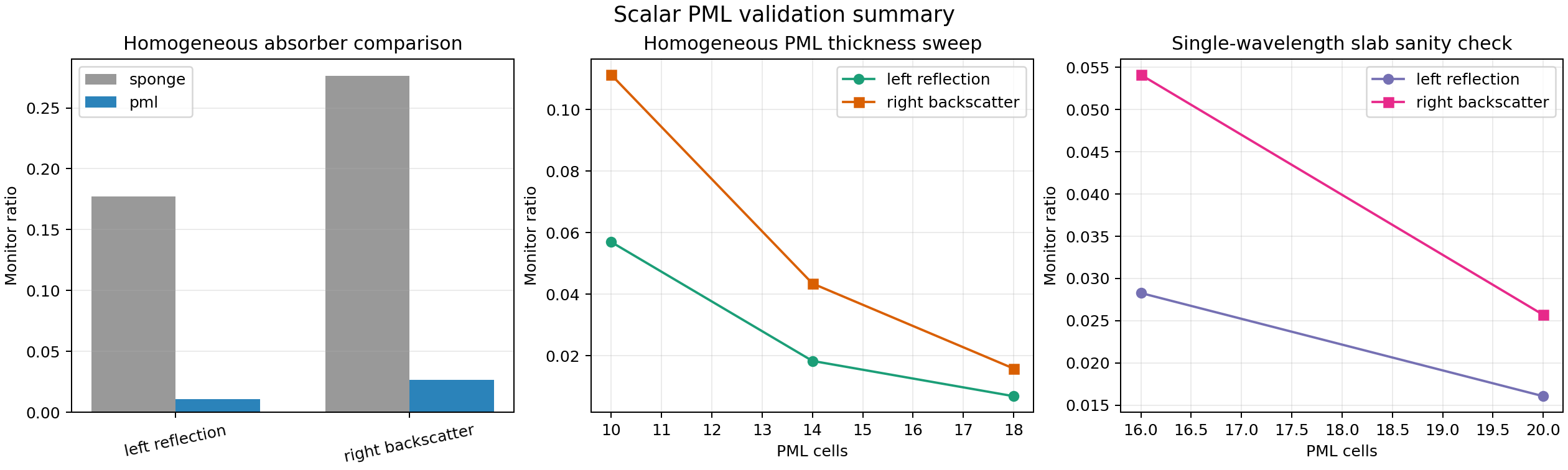
where $s_x$ and $s_y$ are the complex stretching functions. This is not a general Maxwell PML — it is specifically derived for the current scalar Helmholtz formulation, and the outer boundary is still Dirichlet-terminated. But it is materially better than the legacy sponge on the current benchmark. The left reflection ratio drops from 0.1772 to 0.0109 — a 16.3x reduction — and the right-side backscatter ratio drops from 0.2765 to 0.0266, a 10.4x reduction.

Scalar PML vs. legacy sponge on the homogeneous benchmark. The PML reduces backscatter contamination by over an order of magnitude on this test case.

External Validation: The TMM Lesson

Once the absorber was in better shape, I wanted to compare Neon’s outputs against an external analytic reference. The Transfer Matrix Method (TMM) is the natural choice for a slab geometry: it gives exact transmission and reflection coefficients for planar multilayer structures at normal incidence, derivable directly from Maxwell’s boundary conditions [10].

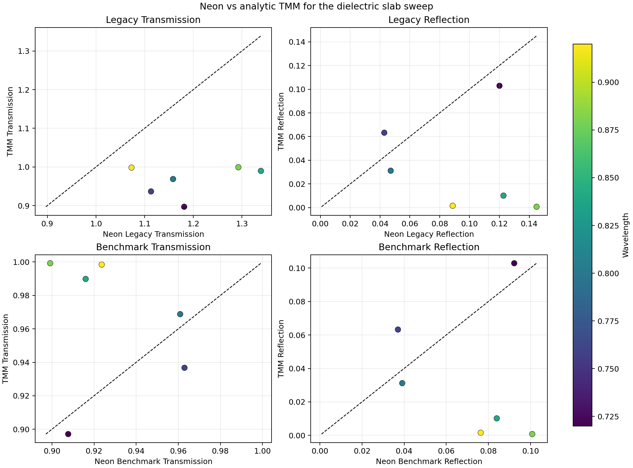
The first comparison failed badly: mean absolute error of 0.228 in transmission. But the failure was instructive. The signed bias was consistently positive — meaning Neon was systematically overestimating transmission relative to TMM, not scattering randomly around the right answer. That pattern is characteristic of a normalization or output-quantity mismatch, not a solver error.

The root cause was that Neon’s transmission and reflection values were monitor-based proxies: local field amplitude samples decomposed heuristically into forward and backward components at a monitor line. These are useful diagnostics, but they are not rigorous flux-normalized power coefficients. After implementing a proper benchmark-facing scalar normalization for the current lossless normal-incidence slab family, the TMM comparison improves to a mean absolute error of 0.0489 and now passes.

Legacy proxy outputs (left) versus benchmark-facing slab coefficients (right) in the TMM comparison. The normalization fix is what moves the comparison from FAIL to PASS — not a solver change.

The lesson is general: output quantity definition matters as much as model architecture when training surrogates. A network trained on a systematically biased output quantity will learn the bias, not the physics.

A cross-check against Ceviche [11] — a differentiable FDFD solver developed by Tyler Hughes and colleagues at Stanford — is less clean. Even after correcting a methodology error (comparing $E_z$ to $E_z$ rather than $E_z$ to $H_z$), the field magnitude correlation is 0.8737. This discrepancy is not yet resolved. It could be grid resolution differences, PML padding mismatches, or source-placement conventions between the two codes. I keep this result in the repository as a documented open question, not a swept-under-the-rug failure.

The ML Layer: Three Models, One Question

The ML experimentation ladder in Neon has three levels, each adding something to the training formulation.

Model A is a small PyTorch MLP taking slab thickness, relative permittivity, and wavelength as inputs and returning transmission, reflection, and peak intensity. No physics in the loss. Trained from scratch on 72 simulation samples from 12 slab designs. This is the baseline against which everything else is measured.

Model B adds a centerline field prediction and a physics-informed loss term: a reduced 1D Helmholtz residual computed along the centerline field, away from crop edges and slab interface points. This connects to the broader PINN framework of Raissi et al. [7] but is deliberately more modest: it applies only along a 1D cropped centerline, not the full 2D domain, and it uses precomputed solver fields rather than requiring the network to satisfy the PDE from scratch.

Model C extends Model B with two additional physics-derived penalties:

A boundary-aware loss that penalizes backward-wave energy in a transmitted-side background window near the PML entrance region, derived from the same forward/backward decomposition used by the solver’s postprocessor.
A source-aware loss that penalizes mismatch to the expected forward plane-wave structure in the source-side background region between the line source and the slab.

Both terms are genuinely physics-derived for this specific setup. Neither is a general Maxwell constraint. But they are real, not decorative.

The trained Neon model released on HuggingFace is the Model C checkpoint. It takes thickness, epsilon, and wavelength as inputs and returns transmission, reflection, and intensity:

from neon import Neon
model = Neon.from_pretrained()
result = model.predict(thickness=0.30, epsilon_real=2.25, wavelength=0.80)
# {"transmission": 0.87, "reflection": 0.09, "intensity": 1.31}

What the Results Actually Say

This is where the project becomes a benchmark platform rather than just a feature stack. The honest answer to “does adding physics to the loss function help?” is: sometimes, and not in the ways you might expect.

The A/B/C Comparison

On the full 72-sample training set, the test mean MAEs are:

Model	Test MAE	OOD MAE
A (baseline)	0.1548	0.2627
B (+ residual)	0.1616	0.2802
C (+ residual + boundary + source)	0.1522	0.2653

Model C improves on both Model B and slightly on Model A on in-domain test error. It also improves on Model B on OOD. But it still does not beat the simple baseline on OOD — a finding that mirrors cautionary results in the broader physics-informed ML literature, where Krishnapriyan et al. [12] showed that naive PINN formulations can fail on relatively simple problems, and where Wang et al. [13] demonstrated that gradient pathologies in multi-term losses can prevent physics terms from contributing meaningfully.

The Ablation: What Is Actually Doing the Work

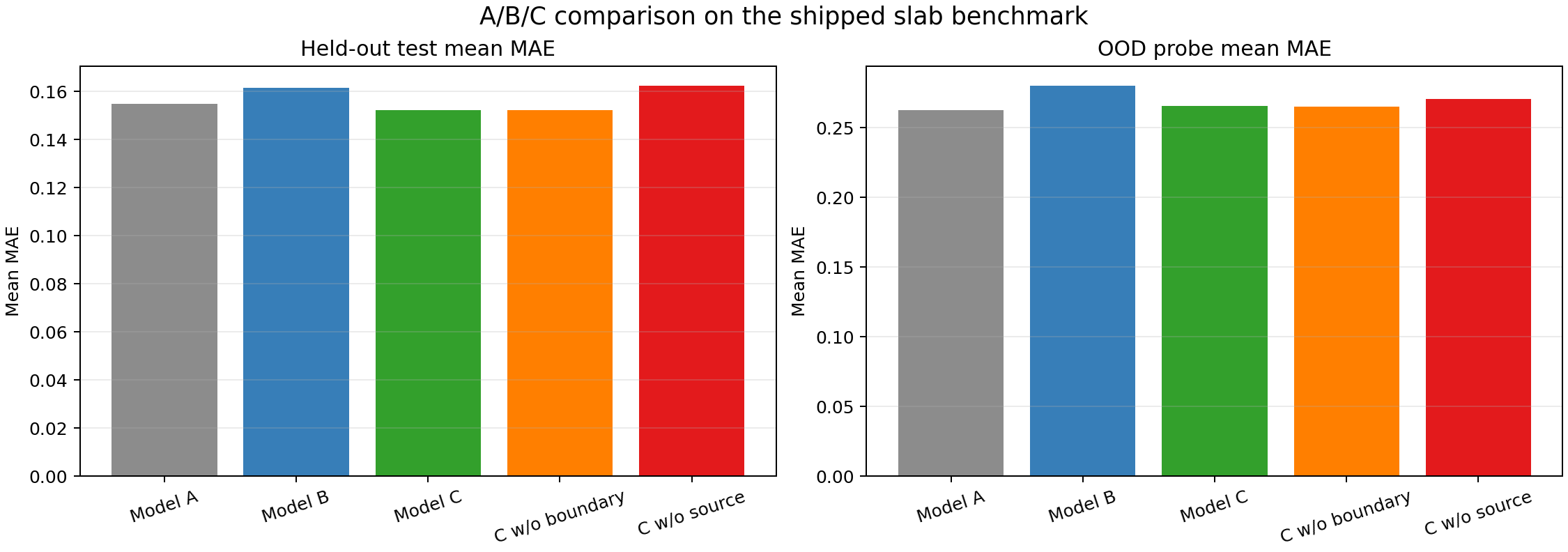
The component ablation is more informative than the headline comparison. Removing the source-aware term from Model C degrades test MAE from 0.1522 to 0.1625 and OOD MAE from 0.2653 to 0.2704. Removing the boundary-aware term changes almost nothing: 0.1522 to 0.1521 on test, 0.2653 to 0.2651 on OOD.

The source-aware term is doing real work. The boundary-aware term is nearly inert at full data.

This is a specific, interpretable finding. The source geometry — knowing where energy enters the domain, and what structure it should have there — is informative supervision that the data alone does not fully provide. The absorber-adjacent region, by contrast, does not carry enough additional signal beyond what the scalar targets already encode, at least in this reduced formulation.

This pattern connects to broader observations in the ML-for-PDE literature. Lagaris et al.’s original neural network approach to boundary value problems [14] showed that boundary conditions are often the hardest part to enforce. In Neon’s case, the source boundary is harder to ignore (it drives the whole field) and so a source-consistency penalty has more leverage than an absorber-exit penalty.

A/B/C comparison including component ablations. The source-aware term is the main active physics contribution; the boundary-aware term shows minimal effect at full data.

The Reduced-Data Study

The reduced-data ablation sweeps training set sizes from 2 to 12 slab designs across three random seeds:

Train Designs	Model A MAE	Model B MAE	Model C MAE
2	0.1723	0.1712	0.1734
4	0.1490	0.1392	0.1394
6	0.1673	0.1591	0.1579
8	0.1657	0.1651	0.1628
10	0.1640	0.1645	0.1623
12	0.1548	0.1616	0.1522

Model C beats Model B in 4/6 settings and beats Model A in 5/6 settings on in-domain test error. But at 2 training designs, Model C is worse than both. This is consistent with the known behavior of physics-informed losses identified by Rathore et al. [15]: physics constraints require enough data to orient themselves. In the extreme low-data limit, the regularization term competes with rather than complements the data term, because the network has not seen enough examples to place the physics constraint meaningfully in parameter space.

Model C beats Model A on OOD in exactly 0/6 settings. This is the most important result in the table. The physics terms help in-domain. They do not solve the extrapolation problem.

Uncertainty and Active Learning

The more recent additions to Neon address a different question: not whether to add physics to the loss, but whether the surrogate can tell you when not to trust it.

Deep Ensembles

The uncertainty approach follows Lakshminarayanan, Pritzel, and Blundell’s deep ensemble method [16]: train five independent MLPs with different random seeds, and use their disagreement as a proxy for predictive uncertainty. This is computationally cheap, does not require architectural changes, and has been shown to produce better-calibrated uncertainty than many more complex Bayesian approaches on tabular regression problems.

The current 5-member ensemble results are:

Model	Test MAE	OOD MAE	Test σ	OOD σ
A ensemble	0.1123	0.1172	0.0086	0.0212
C ensemble	0.1155	0.1293	0.0129	0.0258

Predictive spread does rise on OOD inputs for both models — the right qualitative behavior. But the uncertainty-error correlation is weak and inconsistent: -0.0087 on test for Model A, 0.2458 on OOD for Model C. This means the ensembles are useful as heuristics but cannot be described as calibrated in the sense of Kuleshov, Fenner, and Ermon [17], where calibration requires that stated confidence intervals actually contain the true value at the stated frequency.

Active Learning

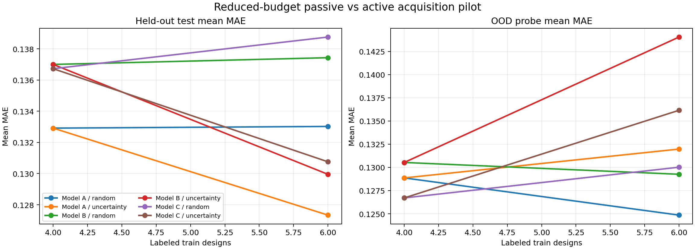
The active learning workflow follows the standard uncertainty-guided acquisition approach: at each round, evaluate ensemble uncertainty across the full parameter grid, run the direct solver on the highest-uncertainty configuration, add that sample to the training set, and retrain. This connects to the broader active learning literature summarized by Settles [18] and to recent work on active learning for scientific simulation by Lookman et al. [19].

The shipped comparison uses one acquisition seed, 4 initial training designs, and one round adding 2 more designs — a deliberately reduced budget, reported honestly as a pilot rather than a full study.

Results at this budget:

Model	Test MAE (active)	Test MAE (passive)	OOD MAE (active)	OOD MAE (passive)
A	0.1273	0.1330	0.1320	0.1249
B	0.1300	0.1374	0.1440	0.1293
C	0.1308	0.1388	0.1362	0.1300

Active acquisition improves in-domain test MAE for all three models. It hurts OOD MAE for all three. And the interaction between physics-informed losses and active learning is essentially neutral: Model C’s test-gain advantage over Model B from active acquisition is only +0.0003.

This is a genuine null result. It suggests the two mechanisms — physics regularization and intelligent data collection — address different aspects of the problem without compounding. Whether this holds at larger acquisition budgets and more seeds is an open question and a primary motivation for the paper.

Passive versus uncertainty-guided acquisition at reduced budget. Active acquisition helps in-domain and hurts OOD across all three model families.

Inverse Design: When Better Accuracy Does Not Mean Better Designs

The inverse design workflow in Neon is deliberately simple: evaluate a dense grid of slab parameters with the surrogate, rank candidates by predicted target proximity, and rerun the top candidates with the direct solver. This follows the spirit of Malkiel et al.’s surrogate-guided design screening [20], with the important addition that all reported design objectives come from direct solver reevaluation, never from the surrogate itself.

The A/B/C design comparison produces an unexpected result:

Model	Best Direct Objective
A (baseline)	0.4732
B (current hybrid)	0.1653
C (enhanced hybrid)	0.4238

Model B — which has worse held-out MAE than Model C — produces the worst design candidate. Model A and Model C both find better designs. This decoupling of surrogate accuracy from design utility is not unique to Neon. Garnett [21] discusses the general problem of acquisition functions in Bayesian optimization that optimize for prediction accuracy rather than design objectives, and similar disconnects have been noted in materials discovery contexts by Pyzer-Knapp et al. [22].

The uncertainty-aware ranking using ensemble disagreement as a conservative acquisition criterion nudges the best Model C candidate from 0.5462 (single-model ranking) to 0.5364 (ensemble-conservative ranking) — a small improvement, but in the right direction. More importantly, it demonstrates that uncertainty estimates are at least directionally useful for design ranking even when they are not fully calibrated for error prediction.

What Is Still Not Solved

Honest accounting of what Neon has not solved is as important as reporting what it has.

The OOD problem is unsolved. No combination of physics losses, ensemble uncertainty, or active learning in Neon’s current formulation reliably improves OOD generalization over the simple baseline. This is consistent with theoretical arguments in the distribution shift literature — Quinonero-Candela et al. [23] — that generalization beyond the training distribution requires either structural inductive biases that match the test distribution, or explicit out-of-distribution data during training. Neither is present in Neon’s current setup.

The Ceviche cross-check is unresolved. A corrected $E_z$-to-$E_z$ comparison still yields a field magnitude correlation of 0.8737. This is documented and tracked, not closed.

The active learning study is a pilot. One seed, one acquisition round, 3-member ensembles. The broader question — whether uncertainty-guided acquisition produces qualitatively different training distributions that improve OOD behavior at larger budgets — requires the multi-seed, multi-round study described in the paper.

The physics losses are still reduced. The centerline residual is 1D, not 2D. The boundary and source penalties apply to cropped background windows, not the full domain. Extending these to full-domain constraints — or to a coarse-solver-plus-learned-correction formulation as explored by Bar-Sinai et al. [24] in fluid dynamics — is the natural next step.

Why This Direction Matters

Most surrogate modeling papers in photonics are asking: how accurate is our model? Neon is asking something harder: does this training pipeline produce a model you can actually trust?

Those are different questions. Accuracy on a held-out test set tells you how well the model interpolates within the training distribution. Trust requires knowing how the model behaves at the boundary of that distribution, what the uncertainty estimates actually mean, whether design objectives derived from the model match direct simulation verification, and whether the physics constraints are doing genuine work or just adding complexity.

The answer Neon gives to these questions is mixed, carefully documented, and I think more useful than a clean positive result would have been. The source-aware physics term helps. The boundary-aware term barely does. Active learning improves in-domain accuracy and hurts OOD robustness at small budgets. Better surrogate MAE does not guarantee better design ranking. Ensemble spread rises on OOD inputs but is not calibrated.

That is what an honest benchmark looks like.

What Comes Next: The Paper

A paper is now in preparation:

Toward Trustworthy Surrogate Models for Electromagnetic Simulation: A Systematic Evaluation of Physics-Informed Training, Uncertainty, and Active Learning on a Controlled Benchmark

The paper extends the active learning study to multiple seeds and larger acquisition budgets, adds proper calibration curves for the ensemble uncertainty, investigates the Ceviche discrepancy, and formalizes the A/B/C comparison results. The central argument is the one this post has been building toward: the relevant question for simulation-driven surrogate modeling is not accuracy but trustworthiness, and answering it requires the kind of controlled, ablation-driven evaluation that most papers in this space do not currently do.

Neon’s Model

The codebase is live at https://github.com/Herr-Professor/Neon.

The trained Neon model — the best Model C checkpoint from the benchmark study — is available at https://huggingface.co/Herrprofessor/Neon. The full benchmark checkpoint bundle including ensembles and evaluation summaries is at https://huggingface.co/Herrprofessor/neon-slab-models. The slab datasets used for training are at https://huggingface.co/datasets/Herrprofessor/Neon-Slab-Datasets.

The model takes dielectric slab parameters and returns optical response predictions in milliseconds:

from neon import Neon

model = Neon.from_pretrained()
result = model.predict(thickness=0.30, epsilon_real=2.25, wavelength=0.80)
print(result)
# {"transmission": 0.87, "reflection": 0.09, "intensity": 1.31}

It is not a general photonics model. It covers one geometry class: a rectangular dielectric slab at normal incidence in vacuum, within the parameter ranges described in the repository. Inputs outside that range will trigger a warning. For researchers working with this class of problem — as a fast screener, a baseline comparison, or a reproducibility tool for the paper results — it is a real, usable predictor. For anything else, use the direct solver.

References

[1] Peurifoy, J., Shen, Y., Jing, L., Yang, Y., Cano-Renteria, F., DeLacy, B. G., … & Soljačić, M. (2018). Nanophotonic particle simulation and inverse design using artificial neural networks. Science Advances, 4(6), eaar4206.

[2] Oskooi, A. F., Roundy, D., Ibanescu, M., Bermel, P., Joannopoulos, J. D., & Johnson, S. G. (2010). Meep: A flexible free-software package for electromagnetic simulations by the FDTD method. Computer Physics Communications, 181(3), 687–702.

[3] Lanteri, S., Scheid, C., & Viquerat, J. (2013). Analysis of a generalized dispersive model coupled to a DGTD method with application to nanophotonics. SIAM Journal on Scientific Computing, 39(3), A831–A859. See also: https://diogenes.inria.fr/

[4] Liu, Z., Zhu, D., Rodrigues, S. P., Lee, K. T., & Cai, W. (2018). Generative model for the inverse design of metasurfaces. Nano Letters, 18(10), 6570–6576.

[5] Wiecha, P. R., Arbouet, A., Girard, C., & Muskens, O. L. (2021). Deep learning in nano-photonics: overcoming the computational bottleneck for electromagnetic inverse design using neural networks. Photonics Research, 9(5), B182–B202.

[6] So, S., Mun, J., & Rho, J. (2020). Simultaneous inverse design of materials and structures via deep learning: Demonstration of dipole resonance engineering using core–shell nanoparticles. ACS Applied Materials & Interfaces, 11(24), 24264–24268.

[7] Raissi, M., Perdikaris, P., & Karniadakis, G. E. (2019). Physics-informed neural networks: A deep learning framework for solving forward and inverse problems involving nonlinear partial differential equations. Journal of Computational Physics, 378, 686–707.

[8] Bérenger, J. P. (1994). A perfectly matched layer for the absorption of electromagnetic waves. Journal of Computational Physics, 114(2), 185–200.

[9] Chew, W. C., & Weedon, W. H. (1994). A 3D perfectly matched medium from modified Maxwell’s equations with stretched coordinates. Microwave and Optical Technology Letters, 7(13), 599–604.

[10] Born, M., & Wolf, E. (1999). Principles of Optics: Electromagnetic Theory of Propagation, Interference and Diffraction of Light (7th ed.). Cambridge University Press.

[11] Hughes, T. W., Minkov, M., Williamson, I. A., & Fan, S. (2019). Adjoint method and inverse design for nonlinear nanophotonic devices. ACS Photonics, 5(12), 4781–4787. See also: Minkov, M., Williamson, I. A., Andreani, L. C., Gerace, D., Lou, B., Song, A. Y., … & Fan, S. (2020). Inverse design of photonic crystals through automatic differentiation. ACS Photonics, 7(7), 1729–1741.

[12] Krishnapriyan, A., Gholami, A., Zhe, S., Kirby, R., & Mahoney, M. W. (2021). Characterizing possible failure modes in physics-informed neural networks. Advances in Neural Information Processing Systems, 34, 26548–26560.

[13] Wang, S., Teng, Y., & Perdikaris, P. (2021). Understanding and mitigating gradient flow pathologies in physics-informed neural networks. SIAM Journal on Scientific Computing, 43(5), A3055–A3081.

[14] Lagaris, I. E., Likas, A., & Fotiadis, D. I. (1998). Artificial neural networks for solving ordinary and partial differential equations. IEEE Transactions on Neural Networks, 9(5), 987–1000.

[15] Rathore, P., Lei, W., Frangella, Z., Lu, L., & Udell, M. (2024). Challenges in training PINNs: A loss landscape perspective. arXiv preprint arXiv:2402.01868.

[16] Lakshminarayanan, B., Pritzel, A., & Blundell, C. (2017). Simple and scalable predictive uncertainty estimation using deep ensembles. Advances in Neural Information Processing Systems, 30.

[17] Kuleshov, V., Fenner, N., & Ermon, S. (2018). Accurate uncertainties for deep learning using calibrated regression. International Conference on Machine Learning, 2796–2804.

[18] Settles, B. (2009). Active learning literature survey. University of Wisconsin–Madison Department of Computer Sciences, Technical Report 1648.

[19] Lookman, T., Balachandran, P. V., Xue, D., & Yuan, R. (2019). Active learning in materials science with emphasis on adaptive sampling in experimental design for efficiency. npj Computational Materials, 5(1), 21.

[20] Malkiel, I., Mrejen, M., Nagler, A., Arieli, U., Wolf, L., & Suchowski, H. (2018). Plasmonic nanostructure design and characterization via deep learning. Light: Science & Applications, 7(1), 60.

[21] Garnett, R. (2023). Bayesian Optimization. Cambridge University Press.

[22] Pyzer-Knapp, E. O., Li, K., & Aspuru-Guzik, A. (2015). Learning from the Harvard Clean Energy Project: The use of neural networks to accelerate materials discovery. Advanced Functional Materials, 25(41), 6495–6502.

[23] Quiñonero-Candela, J., Sugiyama, M., Schwaighofer, A., & Lawrence, N. D. (Eds.). (2009). Dataset Shift in Machine Learning. MIT Press.

[24] Bar-Sinai, Y., Hoyer, S., Hickey, J., & Brenner, M. P. (2019). Learning data-driven discretizations for partial differential equations. Proceedings of the National Academy of Sciences, 116(31), 15344–15349.

Nanophotonics - Light at the Edge of the Invisible

2026-03-22T00:00:00+00:00

"Light is not merely what we see by - it is one of matter's most versatile messengers, and nanophotonics is about learning how to intercept, compress, and redirect that message at extraordinarily small scales."

01 - Introduction

What is Nanophotonics?

Nanophotonics, sometimes called nano-optics, is the study and manipulation of light using structures measured in nanometers, typically from a few nanometers up to roughly the wavelength scale. A human hair is about 80,000 nanometers wide. Nanophotonics works in a regime so small that ordinary far-field optical intuition starts to fail.

Classical optics explains reflection, refraction, focusing, and image formation with remarkable power. But when optical structures shrink toward or below the wavelength of light, geometry, material response, near-field coupling, and sometimes quantum effects begin to dominate. The result is a different design space entirely: one in which light can be confined more tightly, routed more precisely, and coupled more efficiently to matter than conventional lenses and mirrors allow.

This is the territory of nanophotonics. It sits at the intersection of electromagnetism, materials science, nanofabrication, and quantum engineering. Researchers in the field build surfaces, cavities, particles, and waveguides that can squeeze optical fields into deep-subwavelength volumes, guide photons through patterned chips, and tailor how emitters absorb or release light.

Key Concept - The Diffraction Limit

In conventional far-field optics, the diffraction limit prevents light from being focused to an arbitrarily small spot. For visible wavelengths, that usually means a best-case focal size on the order of a few hundred nanometers. Nanophotonics gets around this not by violating Maxwell's equations, but by exploiting near-field coupling, plasmonic confinement, resonant nanostructures, and engineered materials.

02 - The Physics

The Mechanisms Beneath the Surface

Nanophotonics is not one trick or one material platform. It is a collection of physical mechanisms that let researchers manipulate electromagnetic fields beyond the reach of conventional optics.

Electromagnetic spectrum - common nanophotonic operating range

Typical nanophotonic range (UV to near-IR)

Gamma X-ray UV Visible Near-IR Mid-IR Microwave Radio

MECHANISM 01

Surface Plasmon Resonance

At a metal surface, light can drive collective oscillations of electrons known as plasmons. In metallic nanoparticles and nanogaps, these resonances can generate intense local fields and confinement well below the diffraction limit, which is why plasmonics is central to nanoscale sensing and spectroscopy.

MECHANISM 02

Photonic Bandgaps and Crystal Engineering

Photonic crystals are periodic dielectric structures that shape how light propagates. By engineering a photonic bandgap, researchers can block certain wavelengths, create compact cavities, and guide light through patterned defects with high precision and, in well-designed structures, low loss.

MECHANISM 03

Near-Field Optics

Very close to a source or surface, light behaves differently from the propagating waves familiar from ordinary imaging. Near-field optical techniques can resolve features well below the diffraction limit, with 10-20 nm resolution common in advanced implementations and even finer performance possible in specialized systems.

MECHANISM 04

Mie Resonances in Dielectrics

High-index dielectric nanoparticles can support strong resonances without the absorption penalty of metals. Silicon and titanium-dioxide resonators, for example, can shape electric and magnetic optical responses simultaneously, making them attractive for metasurfaces, imaging components, and low-loss nanophotonic devices.

MECHANISM 05

Quantum Confinement

When semiconductors shrink to nanocrystal dimensions, electronic energy levels become quantized. In quantum dots, the emission wavelength can be tuned by size, composition, and structure, which is why they are useful for displays, lasers, imaging probes, and single-photon platforms.

MECHANISM 06

Metamaterials and Metasurfaces

Metamaterials use carefully patterned subwavelength structures to create optical responses not found in ordinary bulk materials. Their two-dimensional cousins, metasurfaces, can replace bulky optics with flat devices that focus, steer, or shape light on a surface only hundreds of nanometers thick.

1-10 nm

Light confinement reported in plasmonic nanogaps

10-20 nm

A representative near-field optical imaging scale

>100 GHz

Bandwidth demonstrated in advanced nanophotonic modulators

1987

Foundational year for photonic bandgap proposals

03 - Brief History

A Field Born From Curiosity

Nanophotonics did not arrive in a single leap. It emerged as theory, microscopy, nanofabrication, and semiconductor processing gradually converged to make nanoscale optical structures both understandable and manufacturable.

1873

Abbe Diffraction Limit

Ernst Abbe formalizes the resolution limit of classical optical microscopy, establishing the barrier later generations would spend decades trying to work around.

1908

Mie Scattering Theory

Gustav Mie derives exact solutions for the scattering of electromagnetic waves by spherical particles, laying mathematical foundations that still underpin nanoparticle optics.

1974

Discovery of SERS

Surface-enhanced Raman scattering reveals that rough metallic surfaces can amplify local fields dramatically, foreshadowing the power of plasmonic confinement.

1981

Scanning Tunneling Microscopy

Atomic-scale imaging becomes practical, making the nanoscale experimentally tangible rather than purely theoretical.

1987

Photonic Bandgap Proposals

Eli Yablonovitch and Sajeev John independently publish seminal papers arguing that structured dielectrics can control the optical density of states and localize light in powerful new ways.

1998

Extraordinary Optical Transmission

Thomas Ebbesen and colleagues show that metallic films pierced with subwavelength hole arrays can transmit far more light than classical aperture theory predicts, energizing plasmonics.

2000s

Quantum Dots Go Commercial

Quantum-dot materials move from laboratory research into displays, imaging tools, and light-emitting technologies, proving that nanoscale optical engineering can scale into real products.

2010s to Present

Metalenses, Silicon Photonics, Integrated Optics

Flat optics, photonic chips, compact modulators, and nanostructured sensors move from demonstration to deployment in data links, imaging systems, sensing platforms, and advanced computation research.

04 - Real-World Impact

Where Nanophotonics Meets the World

Nanophotonics is no longer just a laboratory discipline. It is increasingly a platform technology: one that shows up quietly inside devices for communication, imaging, sensing, and information processing.

🔬

Medical Diagnostics and Biosensing

Plasmonic and nanophotonic biosensors can detect tiny refractive-index changes and weak spectroscopic signals, making them promising for compact diagnostic systems. The long-term appeal is obvious: highly sensitive detection in devices far smaller than conventional benchtop optical instruments.

💻

Optical Interconnects and Computing

Silicon photonics is already replacing some electrical interconnects in bandwidth-hungry environments. Beyond communication, research prototypes in optical and photonic neural computing have reported throughput from the tens to hundreds of tera-operations per second, though the practical comparison to electronic systems still depends strongly on task and architecture.

🌞

Solar Energy Harvesting

Nanostructured surfaces and resonators can trap and recycle light inside thin photovoltaic layers, increasing effective absorption without simply making the device thicker. That matters most for lightweight or flexible solar technologies, where material thickness is expensive.

📷

Flat Optics and Metalenses

Metasurface lenses can focus and shape light in an ultrathin format, offering an alternative to the thick stacks of curved glass used in conventional optics. They are especially attractive where size, weight, and integration matter, such as compact cameras, augmented reality hardware, and miniature imaging systems.

🔐

Quantum Communication

Nanophotonic cavities and waveguides can strengthen the interaction between single photons and quantum emitters. That makes them relevant to quantum repeaters, on-chip quantum optics, and quantum key distribution, where the goal is not magical invulnerability but information-theoretically secure protocols implemented with carefully engineered hardware.

🚗

LiDAR and Autonomous Sensing

Solid-state beam steering based on nanophotonic optical phased arrays could eventually replace bulkier moving-part LiDAR assemblies. If those systems mature, they offer a path toward smaller, faster, and potentially more manufacturable sensing stacks.

05 - Open Challenges

What Remains Unsolved

For all its promise, nanophotonics still faces hard physical and engineering limits.

Ohmic loss in metals remains a central problem for plasmonics. The same free electrons that make metallic confinement possible also dissipate energy as heat, which is a serious penalty for long propagation distances and low-power devices.

Fabrication precision and scalability are equally important. Many high-performance devices demand feature sizes in the tens of nanometers or below. That is feasible in research settings, but reproducible, high-yield, low-cost manufacturing is much harder.

Integration with electronics is one of the field's great commercial opportunities and one of its messiest engineering challenges. Efficient coupling, thermal management, packaging, and co-design with electronics all matter as much as the optical device itself.

Quantum coherence remains delicate. Nanophotonic quantum devices are highly sensitive to disorder, charge noise, surface defects, and thermal fluctuations, which makes room-temperature, scalable quantum photonic hardware a difficult target.

Frontier Watch - Topological Photonics

Topological photonics is often presented as a route to defect-immune transport, and it is an exciting direction. But the strongest version of that claim is not settled. Recent experiments on valley-Hall photonic waveguides have shown that topological design can improve robustness in some cases while still suffering measurable backscattering and propagation loss. In other words: promising, but not a free pass around absorption, fabrication disorder, or all defect classes.

06 - What Comes Next

The Future Is Photonic

The broad direction is clear even if the timeline is not: more of the functions once handled by bulky optics or electrical wiring are moving into compact photonic structures patterned directly onto chips and surfaces.

Photonic neural and analog processors are a compelling example. Several research systems now report very high throughput and energy efficiency in specialized workloads, suggesting that optical hardware may become an important complement to electronic accelerators in bandwidth-intensive tasks.

Nano-optomechanics is another frontier, coupling optical fields to mechanical motion so strongly that tiny resonators can be cooled, measured, and controlled at or near the quantum regime. That could matter for sensing, transduction, and hybrid quantum systems.

Active metasurfaces are moving beyond static flat optics. By combining nanostructures with tunable materials, researchers are building surfaces that can steer beams, refocus, or reconfigure their optical function dynamically.

The bolder historical claim is still worth making carefully: if the twentieth century was shaped by mastering electrons in semiconductors, part of the twenty-first may be shaped by mastering photons in nanostructures.

07 - Selected References

Where These Ideas Come From

This essay is written as a high-level science article rather than a technical review, but the key claims above were tightened against foundational and recent primary sources.

Eli Yablonovitch, "Inhibited Spontaneous Emission in Solid-State Physics and Electronics" (1987), Physical Review Letters.
Sajeev John, "Strong localization of photons in certain disordered dielectric superlattices" (1987), Physical Review Letters.
Thomas W. Ebbesen et al., "Extraordinary optical transmission through sub-wavelength hole arrays" (1998), Nature.
Sara Ek et al., "Slow-light-enhanced gain in active photonic crystal waveguides" (2014), Nature Communications.
Thomas Barczyk et al., "Observation of strong backscattering in valley-Hall photonic topological interface modes" (2023), Nature Photonics.
Xing Lin et al., "11 TOPS photonic convolutional accelerator for optical neural networks" (2021), Nature.
Cheng Guo et al., "Scalable photonic reservoir computing for parallel machine learning tasks" (2025), Nature Communications.
Guilherme Almeida et al., "InP colloidal quantum dots for visible and near-infrared photonics" (2023), Nature Reviews Materials.

Optical Neural Networks - Where the Matmul Is the Hardware

2026-03-22T00:00:00+00:00

Strip away the optics jargon and the cleanest mental model is this: an optical neural network offloads some linear algebra into a physical system where light propagation performs the transform. The interesting engineering question is not whether photons are fast. It is where the digital-analog boundaries, calibration loops, and programmability costs move.

Scope. This post focuses on current inference-oriented ONN hardware, especially coherent Mach-Zehnder-interferometer meshes and diffractive optical systems. Several performance figures below come from different papers and counting conventions, so any GPU comparison is directional rather than apples-to-apples.

00 / Mental Model

Where the linear map becomes physical

An ONN is not “PyTorch, but with lasers.” The more accurate picture is that some learned linear transforms are compiled into a physical scattering network. In a coherent MZI mesh, phase shifters and beam splitters implement a programmable optical transform. In a passive diffractive network, the geometry of stacked phase masks does the work. Either way, the weights are no longer fetched from HBM on every inference.

GPU forward pass

Load weights, run kernels, write activations

The dominant systems story is data movement: weights come out of HBM, are staged closer to arithmetic units, a fused kernel runs, then activations go back to memory. The bottleneck is often memory bandwidth and orchestration more than multiply-add itself.

# each layer: data movement + compute y = relu(x @ W + b) # W is a tensor loaded from memory

ONN forward pass

Encode, propagate, detect

The optical core applies a programmed physical transform to an encoded optical field. For coherent meshes that transform is typically unitary or built from unitary blocks plus amplitude control. For diffractive systems it is set by the masks or metasurfaces in the beam path.

# weights live in optical elements y = detect(propagate(encode(x))) # "loading weights" means setting phases or fabricating masks

        Key systems insight. For the optical linear stage, the model parameters are embodied in hardware state rather than streamed from HBM on each inference. That shifts the bottleneck toward modulators, photodetectors, ADC/DAC precision, calibration, and control electronics.
      

Where this fits in a modern ML stack

Stack layer	Status in an ONN deployment
Your inference harness	Mostly unchanged. You still batch, schedule, validate, and monitor requests in software.
Model parameter artifacts	Compiled to phase settings, mask states, or other hardware control values instead of only tensor checkpoints.
Linear layers	Candidate for optical execution.
Nonlinearities and control logic	Usually electronic today, although some recent chips integrate limited optical nonlinear functions.

01 / Execution Model

The fast path is optical. The tax is at the boundaries.

End-to-end ONN inference is best understood as a domain-crossing pipeline. Digital inputs have to be encoded into optical amplitude or phase, the optical network applies its linear transform, and the result is measured back into the electrical domain. The optical segment is the part people find exciting. The converters are where a lot of the practical pain lives.

Inference pipeline

Input data Digital features, token embeddings, sensor values, or image patches.

→

DAC + modulator Encode values into optical phase, amplitude, wavelength channels, or time bins.

→

Optical propagation Beam splitters, phase shifters, waveguides, or diffractive masks apply the learned linear map.

→

Photodetector + ADC Measure intensity or interference outputs and bring them back to digital logic.

→

Output logits Now you can apply thresholding, softmax, routing, or the next hybrid stage.

          Practical bottleneck. Recent integrated photonic accelerator work explicitly includes TX/RX electronics, DACs, driver circuits, photodetectors, TIAs, and ADCs as core system components. For current mixed-signal ONNs, converter precision and interface overhead often dominate the usable accuracy budget more than the underlying optics itself.
        

What the optical core computes

A structured linear transform

In an MZI mesh, the optical field evolution is a matrix transform built from interferometers and phase shifts. In the cleanest setting that is a unitary matrix. General dense real-valued layers usually need extra decomposition steps, diagonal scaling, or hybrid surrounding circuitry.

What still stays hard

Nonlinear activation layers

ReLU, softmax, masking, and many control-heavy operations are still typically executed in electronics. Some chips now integrate optical nonlinearities, but that is not yet the dominant deployment model. For many systems, every deep layer still pays an optical-electrical round-trip.

02 / Architectures

The backend choice changes everything

“Optical neural network” names a family of hardware strategies, not a single design. The two most useful buckets for a systems reader are programmable coherent meshes and diffractive free-space systems. There is also a middle zone of reconfigurable diffractive processors that trade away some efficiency or compactness to recover programmability.

Programmable coherent photonics

MZI meshes are the tunable matmul kernel

Shen et al. showed a programmable nanophotonic processor with 56 Mach-Zehnder interferometers for vowel recognition, and the Clements design formalized a compact mesh that can implement arbitrary linear transforms across channels with better robustness to loss than earlier layouts.

Why people like it

Runtime programmability

“Deploying weights” means programming phase shifters or related control elements. That makes MZI hardware closer to a tunable accelerator than a fab-time-fixed optical circuit.

The catch

Calibration and scale

Phase noise, crosstalk, drift, and control complexity grow with chip size. The physics is elegant. The control plane is where scaling gets difficult.

Passive free-space optics

D²NNs are optical inference burned into geometry

Lin et al. introduced diffractive deep neural networks as stacks of passive diffractive layers that collectively implement learned functions at the speed of light. Once those layers are physically made, the base design behaves much more like a write-once inference artifact than a reprogrammable chip.

          Important distinction. The classic D²NN story is passive and largely fixed after fabrication. Reprogrammable spatial-light-modulator or metasurface variants exist, but the base architecture is much closer to ROM than to hot-reloaded GPU weights.
        

Why it is attractive

Huge parallelism in free space

Light diffracts across many spatial degrees of freedom at once, so a single optical pass can process large fields in parallel.

Why it is limiting

One mask stack, one deployed function

If the weights are embodied in fabricated masks, model updates are no longer a software deployment problem. They become a hardware replacement problem.

Middle ground

Reconfigurable diffractive processors recover flexibility

This is the compromise architecture. Instead of a permanently fixed diffractive stack, the optical processor uses reconfigurable elements, such as digital-coding metasurfaces or other optoelectronic control planes, to support different models or tasks. Zhou et al. reported a reconfigurable diffractive processing unit with millions of neurons and adaptive training to compensate system errors.

✓ more flexible than passive D²NN ~ more control overhead ~ still hybrid, not purely passive

03 / Weights & Training

Weights are no longer just tensors

The most unintuitive part for systems engineers is that “model weights” can map to phase settings, mask geometries, or other physical control states. That changes deployment, versioning, evaluation, and reproducibility. It also changes how carefully you have to talk about training: offline simulation is common, but it is no longer the only story.

What a weight means in a coherent ONN

A compiled physical configuration

In an MZI-based design, a learned matrix is decomposed into interferometer parameters and phase values. In a diffractive design, the “weights” are the transmissive or phase profile of each layer. That means deployment artifacts often include both a model checkpoint and a hardware-programming representation.

# Conceptually, one MZI is a tunable 2x2 block def mzi(theta, phi): # beam splitter + phase shift return U(theta, phi) # Full optical layer = product of many such blocks # "Loading weights" = setting phases and calibration state

Common deployment workflow today

step 1

Train or co-train a differentiable optical model

The common path is still digital optimization in PyTorch, JAX, or custom simulators that model the optical layer and its hardware constraints.

step 2

Compile to hardware parameters

For coherent meshes this can involve decompositions such as Clements-style parameterization plus any diagonal scaling and hardware-aware clipping.

step 3

Program or fabricate the optical system

You send voltages to phase shifters, configure a reconfigurable optical front-end, or physically realize a fixed mask stack.

          Correction to a common oversimplification. It is no longer accurate to say ONN training is always offline simulation followed by one-way programming. Pai et al. experimentally demonstrated in-situ backpropagation on a silicon photonic neural network, and Bandyopadhyay et al. showed forward-only in-situ training on a fully integrated chip. Offline compilation is common. It is not the only training mode anymore.
        

What this means for evaluation and reproducibility

Factor	GPU assumption	ONN reality
Model artifact	Tensor checkpoint	Tensor checkpoint plus compiled phase or mask state and calibration metadata
Numeric precision	Bit-defined formats like fp32, bf16, int8	Mixed-signal, often single-digit effective bits at system level
Runtime determinism	Close to bit-exact for fixed seeds and kernels	Affected by drift, noise, bias settings, device mismatch, and readout error
Calibration	Usually not part of model versioning	Operationally important and may change output quality over time
Eval thresholds	Exact-match and narrow tolerances are common	Statistical tolerances and repeated measurements are often more defensible

04 / Performance

The numbers are impressive, but the units need adult supervision

ONN papers often report outstanding latency and energy-efficiency numbers, but comparing them directly to GPUs is tricky because precision, sparsity assumptions, workload shape, and system boundary definitions vary. The right way to read the field is: optical linear algebra can be extraordinarily efficient, but end-to-end usefulness still depends on control electronics and deployment fit.

Taichi chiplet (Science 2024) 160 TOPS/W Reported energy efficiency for a large-scale diffractive-interference hybrid photonic chiplet with millions-of-neurons capability.

PACE system 2.38–4.21 TOPS/W Reported system-level efficiency for a 64 × 64 integrated photonic accelerator, depending on whether laser power is included.

FICONN (Nature Photonics 2024) 410 ps Demonstrated latency for a three-layer fully integrated coherent optical neural network.

PACE system 7.61 bits Average bit accuracy reported for a 64 × 64 integrated photonic accelerator system.

Read each number by its system boundary

This is the part that trips people up. ONN papers, integrated mixed-signal accelerator papers, and vendor GPU spec sheets are usually not measuring the same thing. So compare them as architectural signals, not as interchangeable benchmark rows.

System	Reported number	What to remember
Taichi chiplet	160 TOPS/W	Paper-reported efficiency for a specialized photonic chiplet architecture optimized around optical computing.
PACE 64 × 64 accelerator	2.38 TOPS/W including lasers, 4.21 TOPS/W excluding lasers	Integrated mixed-signal system number, not just an isolated optical core.
FICONN	410 ps latency	Latency number on a compact fully integrated coherent ONN, useful for understanding the speed floor of the optical path.
H100 SXM	Up to 1,979 TFLOPS BF16/FP16 with sparsity, 3.35 TB/s HBM, up to 700 W	Vendor peak spec for a general-purpose GPU. This is the machine you already know, but it is not a like-for-like paper boundary.

Why people keep saying ONNs dodge the memory wall

# GPU intuition flops = 2 * N * M bytes = N * M * dtype_size # weight traffic arithmetic_intensity = flops / bytes # ONN intuition for the optical linear map # weights are embodied in phase settings / optical structure # per-inference weight traffic is reduced or eliminated at the optical stage # the bottleneck shifts to modulator rate, photodetector chain, ADC/DAC, and control I/O

The claim is directionally right for the optical linear layer, but it should be phrased carefully. End-to-end ONN systems still rely on electronics, control paths, and often repeated domain conversions.

05 / Tradeoffs

Strong in narrow places, weak in exactly the places LLMs care about

The honest assessment is that ONNs are compelling when you can exploit fast, energy-efficient linear transforms with limited need for online updates and with a tolerance for mixed-signal imperfection. They are much less compelling when you need deep stacks of nonlinear layers, exact reproducibility, or massive reprogrammable parameter counts.

Engineering verdict

Dimension	Verdict	Why it matters
Energy per linear op	✓ strong win	Optical propagation is passive or nearly passive compared with electronic MAC arrays.
Latency for linear inference	✓ win	The optical core is extremely fast; integrated systems have already demonstrated sub-nanosecond class latency in small networks.
Precision and reproducibility	× loss	Noise, converter limits, drift, and calibration state make exact-match expectations harder to defend.
Programmability	~ depends	MZI meshes are reconfigurable; passive diffractive networks are much closer to hardware-fused models.
Nonlinear depth	× loss	Hybrid optical-electronic round-trips are still the default for many architectures.
Model size scaling	× loss	Even impressive photonic demonstrations remain far below the parameter counts and memory footprints of frontier LLMs.
Training	~ partial	In-situ training exists in research prototypes, but training is not yet the field’s easiest or most mature deployment story.
Inference-only, fixed-function tasks	✓ best fit	Classification, signal processing, and front-end sensing pipelines are where ONNs look most deployable today.

        Deployment answer today. ONNs look most plausible for latency-critical or energy-sensitive inference where the linear transform dominates and the model changes slowly. They are not a general drop-in replacement for LLM training, online fine-tuning, or giant dynamically updated models.
      

Selected primary sources

Research behind the claims in this explainer

Shen et al. (Nature Photonics, 2017) demonstrated a programmable nanophotonic processor with 56 MZIs for optical neural inference.

Clements et al. (2016) described a compact universal interferometer mesh used heavily in programmable photonics.

Pai et al. (Science, 2023) experimentally realized in-situ backpropagation on a silicon photonic neural network.

Bandyopadhyay et al. (Nature Photonics, 2024) demonstrated a fully integrated coherent optical neural network with forward-only in-situ training and 410 ps latency.

Xu et al. (Science, 2024) reported the Taichi photonic chiplet with 160 TOPS/W and millions-of-neurons capability.

Zhou et al. (Nature Photonics, 2021) reported a reconfigurable diffractive processing unit with adaptive training and millions of neurons.

Lin et al. (Science, 2018 preprint / related DOI) introduced diffractive deep neural networks as passive optical inference stacks.

Liu et al. (Nature Electronics, 2022) demonstrated a programmable diffractive deep neural network based on a digital-coding metasurface array.

An integrated large-scale photonic accelerator with ultralow latency reported a 64 × 64 photonic accelerator system with 7.61-bit average accuracy and explicit TX/RX electronics in the system architecture.

NVIDIA H100 official specifications are used only as a modern GPU orientation point for memory bandwidth and tensor-throughput scale.